Figure 15 depicts results of Ordinary Kriging for effective porosity at five different elevations of the domain. The colored dots in these plots are samples of effective porosity. It is noticeable that there are artifacts and clear boundaries between estimations around the edges of the model. These hard boundaries are the result of Kriging acting as extrapolation rather than interpolation in these sections of the domain, which is due to sparse samples present in those areas. It is usually preferred not to rely too much on these estimations as they are bound to be inaccurate. Similar results are also generated for the three secondary variables using Ordinary Kriging.
Figure 15 - Results of Ordinary Kriging of effective porosity at five different elevations in the domain. Colored dots represent sample locations in the domain and boundaries in the edges of the domain are due to sparse sampling in those sections.
Apart from the actual Kriged values of the four variables, Kriging also generates estimation variances as its result. Estimation variance is a measure of how precise the Kriging result is at each location. It is expected that estimation variance would be low at densely sampled areas and high in sparsely sampled sections; this is due to locations near samples having very high spatial correlation with sample values and thus, having better estimations. Samples are sources of concrete information and having many samples near an unknown location leads to high correlation with those samples and a very low estimation variance at that location. Estimation variances generated by Ordinary Kriging for effective porosity can be seen in figure 16. As was expected, estimation variance is low at and around samples and higher in other areas. Like figure 15, the colored dots in figure 16 represent samples of effective porosity. Similar results were also generated for the three secondary variables.
Figure 16 - Estimation variance of effective porosity in 5 elevations of the domain. Colored dots represent samples of effective porosity. It is clear that estimation variance is low in densely sampled areas and higher in areas further apart from samples.
Having found estimations of the four variables, Collocated Cokriging of effective porosity using the three secondary variables was implemented. Figure 17 shows the results of Ordinary Kriging of effective porosity along with Collocated Cokriging with the three secondary variables at the same elevation of 520 meters. This figure is showing that Collocated Cokriging is generating significantly different results in low-value areas, but generally similar estimations in high-value areas. Another significant difference between the two methods is less smooth results in Collocated Cokriging compared to Ordinary Kriging. Looking at Ordinary Kriging results, much of the map seem to be containing smoothed estimations, with low values and high values showing little difference across the domain. In Collocated Cokriging however, this difference is more significant and the variability between low and high value areas is more noticeable. This additional variability in results of Collocated Cokriging could be due to errors in this method, but it also could be due to Collocated Cokriging performing better in capturing the variability of effective porosity across the domain. Validation and analysis of the results must be implemented before it could be decided which is the case.
Figure 17 - Estimations of effective porosity genrated by Ordinary Kriging (first figure from left), Collocated Cokriging with oil saturation (second figure from left), Collocated Cokriging with effective water saturation (third figure from left), and Collocated Cokriging with bulk mass fraction of oil (fourth figure from left). Colored dots represent samples of effective porosity. All these results are in the elevation of 520 meters.
Figure 18 depicts a comparison between estimation variances produced by the four processes. This figure alone shows that estimation variance has dramatically reduced in Collocated Cokriging compared with Ordinary Kriging. Although in all four models the lower estimation variances are focused around sample locations and high estimation variances are in areas which are far away from samples, this figure shows in the same grid locations Collocated Cokriging is generating less estimation variance than Ordinary Kriging. This figure is clearly showing that Collocated Cokriging is preforming significantly better than Ordinary Kriging in producing lower estimation variances.
Figure 18 - Map of estimation variance generated by (from left to right), Ordinary Kriging, Collocated Cokriging with oil saturation, Collocated Cokriging with effective water saturation, and Collocated Cokriging with bulk mass fraction of oil. Notice how estimation variances have dropped across the domain in the Collocated Cokriging results. In all four plots, lower estimation variances are focused around densely sampled areas.
Although it could be interpreted from figure 18 that Collocated Cokriging is generating lower estimation variance across the domain, it is not clear in which sections and parts this improvement is higher or lower. Figure 19 illustrates the difference between estimation variance of Ordinary Kriging and Collocated Cokriging with the three secondary variables at each grid cell. This figure reveals critical information, as it shows that improvement of estimation is highest in areas where samples are most scarce, while some improvement can be seen in more densely sampled areas. Lower estimation variance in areas that are far away from samples and less reliable information is available is revealing that Collocated Cokriging is improving estimations at precisely the areas that this improvement is most needed. Densely sampled areas are already yielding decent estimations (as is evident in figure 18), so an increase in estimation quality in sections with poor estimation results makes a vital positive impact on the overall estimation of the domain.
Figure 19 - The difference between estimation variance of Collocated Cokriging with the three variables and Ordinary Kriging at the 520 meters elevation. High differences are showing high improvements in estimation quality, which are most significant in sparsely sampled sections of the domain.
Although it is clear that estimation variance drops in the three Collocated Cokriging results, it is not clear if these results are respecting global statistical features of effective porosity. As was explained in the methods page, in order to find the true mean and distribution of effective porosity we must implement declustering. Declustering gives us a weighted average of effective porosity (with weights being declustering weights allocated in the process to each sample) and it is important if the average of estimations generated by Kriging or Collocated Cokriging are very close to this declustered average of effective porosity. In case a significant difference exists between these averages, it is showing that estimation method is producing unreliable results. This is based on the theory of Kriging, which like linear regression, produces the best unbiased estimation of a spatial variable. The unbiased aspect of Kriging means the average of estimations produced by Kriging is equal or very close to the average of the spatial variable itself. If this statement is not true for a set of results from a Kriging or Collocated Cokriging process, it is indicating that method is not producing correct results and can not be relied on. This deviation could be due to many reasons, including erroneous variogram models, modelling errors in Kriging, or lack of sufficient samples in the region.
Figure 20 allows us to test whether these four processes have generated results that respect the declustered mean of effective porosity and to further quantify their performance. In the first row, the average estimation variance produced by each of the four estimation processes are listed. This further confirms the observation made from figure 18; estimation variances are significantly less for results from Collocated Cokriging compared to Ordinary Kriging. This also shows that among the three variables, Collocated Cokriging with bulk mass fraction of oil is resulting in lowest estimation variance compared to the other two secondary variables. The second row is also listing the standard deviation of estimation variances for the four processes. Like the average estimation variance, standard deviation of Collocated Cokriging processes are significantly lower compared to Ordinary Kriging, with lowest value for bulk mass fraction of oil. This means that the histograms of all estimation variances produced for the entire domain are much less dispersed for Collocated Cokriging compared to Ordinary Kriging. The combination of the first two lines mean that not only the average of estimation variance is lower for Collocated Cokriging, but their distribution is also less dispersed. This is only indicative of the fact that Collocated Cokriging is generating much more precise results.
Figure 20 - The results of the four processes compared with each other on average estimation variance, standard deviation of estimation variances, and the difference between estimation mean and true mean of effective porosity. The green cells are indicating which process is preforming best in each criterion.
The third line is the difference between average estimations produced by each process and the true mean of effective porosity, calculated by declustering. This difference shows how much the results of each process are in-line with reality. Lower difference means that the average of estimations produced in that process is closer to the true mean of effective porosity, and as a result more unbiased. Although Collocated Cokriging with bulk mass fraction of oil produced much more precise results with lower estimation variances, this line is showing that it has the highest difference with the true mean of effective porosity. The most accurate results in this case are generated by Collocated Cokriging with effective water saturation, followed by Collocated Cokriging with oil saturation, and Ordinary Kriging.
One of the differences between the three secondary variables are their correlation with effective porosity. As was discussed in Kriging theory, correlation between the primary and secondary variables has a direct impact on the estimation of the primary variable in Collocated Cokriging. In theory, the stronger this correlation is, the better are the results from Collocated Cokriging. Figures 21 and 22 illustrate a comparison between the three results generated by Collocated Cokriging with regards to the correlation between the primary and secondary variables. It is clear from these figures that correlation coefficient has an inverse relation with average estimation variance, with higher correlation yielding lower estimation variance. However, this argument does not hold for difference between estimation mean and true mean of effective porosity; in figure 22, the lowest difference is in Collocated Cokriging with effective water saturation that has a lower correlation with effective porosity than bulk mass fraction of oil. This could be due to other factors influencing these models, including variogram models and declustering. Consequently, it cannot be automatically assumed that Collocated Cokriging would generate more accurate results than Kriging and this conditions must be separately checked.
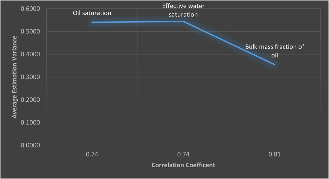
Figure 21 - Average estimation variance of Collocated Cokriging with each of the three variables, plotted with each variables' correlation coefficient with effective porosity. Estimation variance is lower for bulk mass fraction of oil and almost the same for oil saturation and effective water saturation, which have equal correlations with effective porosity.
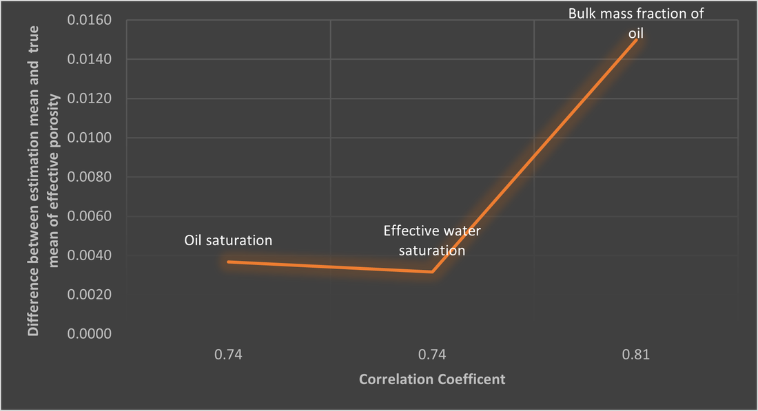
Figure 22 - Difference between estimation mean and true mean of effective porosity, plotted against the correlation coefficient of the secondary variables with effective porosity. Although bulk mass fraction of oil has a higher correlation with effective porosity, it has the highest difference between the three variables which shows its performance being less reliable than the other two variables.
Conclusion
The results of this project reveal a number of important points about Collocated Cokriging and its advantages over Ordinary Kriging. First, Collocated Cokriging proved to decrease estimation variance for every single grid cell in comparison to Ordinary Kriging. This is a significant result and was already expected based on the theory of Kriging.
Second and perhaps more importantly, Collocated Cokriging showed to be decreasing estimation variance at sections of the domain where less samples were available. This important conclusion means Collocated Cokriging improves our estimations in areas where we most need improvement, which is a significant advantage over Ordinary Kriging.
Third, Collocated Cokriging with a secondary variable with a higher correlation with the primary variable leads to lower estimation variances in the results.
Fourth, Collocated Cokriging performs adequately with regards to honoring global statistical features of the target variable. As was seen, the estimation mean for the three Collocated Cokriging processes were very close to the true mean of effective porosity. This confirms that Collocated Cokriging, just like Kriging, is an unbiased linear estimator. However, unlike estimation variance, Collocated Cokriging with a variable with higher correlation did not lead to less error in estimation mean. This conclusion means that honoring target statistics of the variable of interest is dependent on other factors than just correlation between the primary and secondary variables. These factors could be variogram modelling, declustering method, Collocated Cokriging parameter selection, grid cell size, and other decisions.
Overall, Collocated Cokriging proved to be a more reliable and accurate method of spatial estimation in comparison to Ordinary Kriging. If the results generated by Collocated Cokriging respect target statistics of the variable of interest (mean and standard deviation), it should be preferred to Kriging, as it significantly reduces estimation variances and improves the quality of spatial interpolation at areas where fewer samples are available. Besides, variables with a higher correlation to the primary variable generate more precise results and in case they respect global statistical features of the primary variable, they should be prioritized. Improvement in estimation precision, especially in sparsely sampled areas, could remove the need for further sampling in many projects by just using more than one variable at already sampled locations, which is a significant advantage of Collocated Cokriging over Kriging.