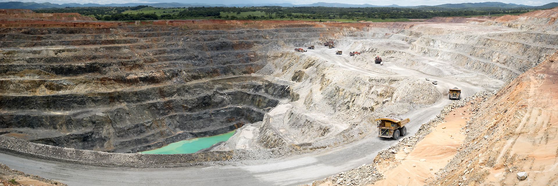
1. Declustering: in a typical mining or petroleum project, samples and boreholes are not collected and drilled equally across the entire domain. Sampling is conducted in separate phases and at each step the focus is on areas of interest, which could be areas that have shown high mineral concentration or hydrocarbon presence. This focus on specific sections of the geological domain leads to high concentrations of samples at those sections and very few samples collected at other areas. This intentional bias in the sampling process has consequences for global statistical features like mean, distribution, and variance of variables. In order to remove this bias in the samples, a process called declustering is implemented, where each sample receives a weight based on how densely sampled is its vicinity. Samples in highly concentrated areas receive lower weights and those in sparsely sampled areas receive high weights. The results of this process yield accurate means and distributions of all variables that are important in the Kriging process.
2. Defining the Grid Cells: in the previous sections, Kriging was referred to as a method that estimates a variable at every location in a domain. In a more precise phrasing of the method, it must be noted that Kriging estimates a variable at certain discretizations of the domain which are referred to as grid cells. Grid cells are defined by a cubic volume with lengths in the three directions (x, y, z). Kriging makes estimations at those cells throughout the entire domain. Figure 04 illustrates a conceptual model of a gridded volume and how each cell receives a single value of the variable. Defining the volume of these grid cells depends on the modelling goals and geological characteristics of the domain. In some geological settings where variables change in very small scales, grid cells must be defined small enough to capture those features. Defining this volume also depends on the available computational capacity. Fine cells result in a larger number of grid cells in a model which increases computational intensity and demand. For this project, a grid cell with dimensions of 50*50*1 meters is defined to discretize the domain.
Figure 04 - A gridded volume where interpolation of a variable is implemented using 5 samples. Notice how the value of the spatial variable is the same at each cell. A cell is the smallest unit in an interpolation problem and interpolated values are allocated to each cell (gisgeography.com)
3. Standardizing the Variables: since different variables are used in relation with each other and these variables have different units, it is important to standardize these variables and transform them back to their original units at the end. Normal score transform is also a possibility but since it is not a linear function, it probably generates bias in the results.
4. Variography: as mentioned in the introduction page, variogram is the measure of spatial correlation between all locations at the subsurface for a specific variable. Variograms are a complex topic and a full explanation of their theory is out of the scope of this project. However, a brief summary on how they are calculated and modelled is presented here.
Referring back to the variance-covariance matrix in figure 2, it is clear that in order to interpolate values of a spatial variable by Kriging we must have access to the covariances between all samples of the variable and every single grid cell in the domain (for the Kriging of each grid cell, that cell becomes the response variable and the samples act as predictor variables). Since all these variables are values of the same spatial variable at different locations in the domain, variogram must produce the covariance between every single grid cell in the domain with any other grid cell; this includes all the samples and the grid cell that they fall into. Having all these covariances, we are able to solve the system of equations in expression 3 for any unknown grid cell. Now the task is clear: finding the spatial covariance between any pair of grid cells at the domain for a spatial variable.
Variogram achieves this task by using the available samples of the spatial variable and inferring a mathematical function which defines the spatial correlation at the domain. Figure 5 illustrates a 2D sample set of effective porosity as an example. In the first step, we must pick the major direction of continuity. This direction is picked based on the geological understanding of the domain and is defined as the direction along which samples show the highest amount of homogeneity and consistency. This could be due to geological and chemical processes that shaped the domain working along that specific direction. In case of figure 5, -45 degrees from North (or the azimuth of 315 degrees) is picked as the major direction of continuity.
In the next step, a lag distance is selected for the data set. This distance is usually picked as the minimum spacing between samples in the data set. Then, all samples that are distanced by that amount in the major direction of continuity are paired with each other (red flashes in figure 5). The pairing process takes place with a certain amount of tolerance with regards to direction and distance; this means that if the lag distance is defined as h and the major direction of continuity as m, samples that are distanced h +/- htol meters from each other and along m +/- mtol degrees are all paired together. These are referred to as tolerance parameters and allow more pairs of samples to be counted in the process (figure 6). Once this process is finished, all the paired points are plotted together in what is called a h-scatter plot which is depicted in figure 7. Values that were found at the tip of the red flashes, called head values, are plotted on the horizontal axis and the tail values are plotted along the vertical axis. As can be seen in figure 7, these points are correlated to each other, since they are all collected as samples with a particular distance from each other; this is a reflection of spatial correlation in the domain.
Figure 05 - a 2D geological setting where samples of effective porosity are taken. Samples are paired along the major direction of continuity and with a specific lag distance. The points that are paired are shown with red flashes (Eidsvik, J. Pyrcz and Deutsch, 2015).
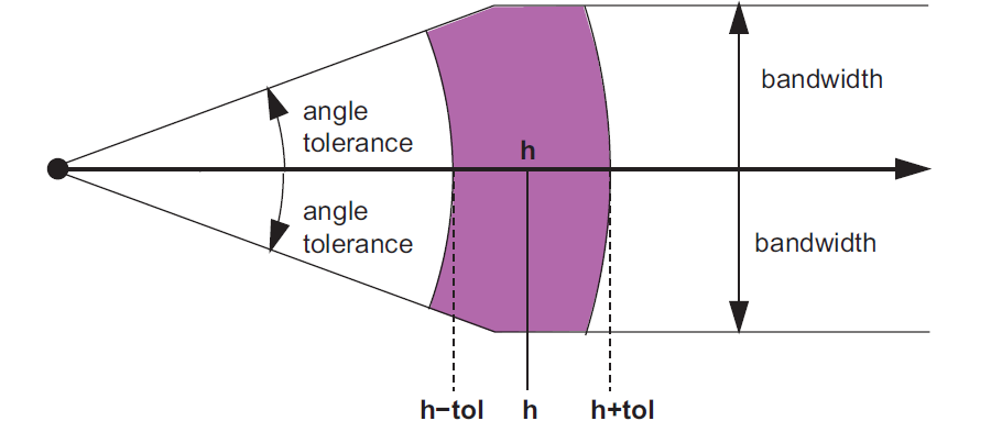
Figure 06 - samples are paired with a degree of tolerance with regards to direction and distance (called angle tolerance and lag tolerance). This allows for more pairs of points to be counted which decreases erratic changes in the variogram. Bandwidths restrict the angle tolerance so that irrelevant points would not be paired together, as distances increase (Eidsvik, J. Pyrcz and Deutsch, 2015).
Figure 07 - a h-scatter plot of all pairs of points with a specific distance and along the major direction of continuity. The correlation between head and tail values is -0.47, which is a reflection of spatial correlation of effective porosity at this domain (Eidsvik, J. Pyrcz and Deutsch, 2015).
This process is repeated for multiplications of the lag distance and each time a new scatter plot is found, just like figure 7. These scatter plots and their correlations are giving a measure of spatial continuity along the major direction. Using expression 6, which gives us the variogram value (γ), we can find the average squared difference for all sample pairs with a lag spacing of h. Finding this value for different lengths of h and along the major direction of continuity result in figure 8, which is called the experimental variogram. As can be seen here, with increasing lag distances the amount of dissimilarly or the variogram value increases. In other words, spatial correlation decreases. This process is repeated for the direction perpendicular to the major direction of continuity, called minor direction of continuity, and in case the data set is 3D, in the vertical direction as well. The results of this process are three experimental variogram plots along these three directions. Finding the variogram value for a distance of h, the spatial covariance of h can be also calculated using expression 7. Subtracting the variogram value of h from the variance of the variable results in the spatial covariance of h. Spatial covariance of h is the amount of covariance of the spatial variable between two points that are distanced h meters from each other. This is the value that is used as input in the Kriging system of equations.
Expression 6:
Figure 08 - Calculating the variogram value for different lag distances of h and along the major direction of continuity results in the experimental variogram (left), where each point represents a scatter plot of all pairs of sample that are distanced h meters apart in that direction (Eidsvik, J. Pyrcz and Deutsch, 2015).
Expression 7:
Referring back to the original problem, variogram must generate covariances between all pairs of grid cells for a spatial variable in the domain. These pairs of points could be connected to each other with a vector that could have any direction and any length. The experimental variogram gives values of spatial correlation for specific lag distances and only along specific directions. The next step requires fitting some known variogram functions on the experimental variogram which enables us to calculate the spatial covariance for all pairs of grid cells in the domain. The result of this process is the variogram model that is illustrated in figure 9. This figure depicts the actual variogram of effective porosity in this project. The points represent the experimental variogram values in the three directions (major, minor, and vertical) and the lines are variogram models that are fit on the experimental variogram points. The variogram model is a mathematical function that allows calculation of all C(h) in any direction and any distance.
Figure 09 - The points are the experimental variogram of effective porosity in the major, minor, and vertical directions. The lines are the variogram models that are fit on these points. The horizontal line drawn at 1.0 is called the variogram sill and represent the variable's variance (standardized). The variogram model is only fit for points below the sill, as points above the sill are values that are above the variance of the variable and have no spatial correlation with each other. The points with a red halo show experimental variogram points that have been calculated with too few pairs of samples and acts as a warning not to use them in the variogram modelling process.
5. Kriging: having found the variogram model in the previous step, it is now time to implement Kriging and generate estimations of the four variables. There are two common methods of Kriging: Simple and Ordinary Kriging. The only difference between these two methods is that in Ordinary Kriging the sum of all weights used in the Kriging of a grid cell is set as 1, which results in removing the mean of the variable from the Kriging equation (expression 8). This is useful as in Simple Kriging an assumption is made that claims the mean of the Kriged variable is constant over the entire domain. This is usually not the case, as variables have different means in different zones of the domain. As a result, it is usually preferred to use Ordinary Kriging as it does not make this assumption and does not require the mean of the variable as an input to the process.
Expression 8:
6. Collocated Cokriging: having the Kriged estimations of the four variables that were produced at step 5, Collocated Cokriging could be implemented. Since the target of this process is effective porosity, the variogram that is used in Collocated Cokriging is the variogram of effective porosity. The process takes the Kriged estimations of the other variables and their correlation with effective porosity as input and generates estimations across the entire domain.
7. Back-transform: since all the variables used in the previous steps were standardized in step 3, the generated results from steps 5 and 6 must be back-transformed into original units. This takes place by multiplying the standard deviation of the variable and adding the mean to all the values.
All the stated processes and methods were implemented in Python 3.0 using the pygeostat package.