In mining and petroleum engineering, one of the main goals is to locate a deposit or a reservoir that is economically profitable to mine and extract. Increasing the precision and the degree of certainty in our understanding of the subsurface generates better and more reliable models of the underground. Such reliable models would bring a better insight into planning of a mineral or oil extraction campaign on the deposit or the reservoir. Apart from increasing the profitability of such extraction campaigns, these precise models reduce the physical distortion of the earth by reducing errors in placement of wells or mine pits. A reduction in physical distortion of the earth significantly decreases adverse environmental effects of a mining or petroleum operation. Because of all these reasons, it is critical to accurately locate a deposit or a reservoir to conduct an efficient mining or petroleum extraction project.
However, in most situations this task is similar to searching for a needle in a haystack; deposits are in order of a few hundred meters to a few kilometers, while regions of study are often in scale of tens of kilometers. So, boreholes (which are vertical holes dug in the ground) must be drilled and samples of spatial variables that guide engineers to concentrations of minerals and hydrocarbons must be taken. But collecting borehole samples is extremely expensive and very few samples could be extracted from the subsurface. Now the issue is to make a comprehensive estimation of the content of the subsurface using very few samples of spatial variables that are available. This is called spatial estimation.
Theoretical Background
A commonly used method of spatial estimation is Kriging. Daniel G. Krige, who was a mining engineer, came up with the theoretical concept of Kriging, which is an extension of linear regression for the purpose of spatial estimation (D.G. Krige, 1952). In a simple linear regression problem, measurements of two different variables are plotted together in a scatter plot with each axis indicating the values of each variable. In case a strong correlation exists between these two variables, they more or less group to form a line which has a slope equal to the correlation coefficient between the two variables. This means that by having measurements of just one variable (the predictor variable), the values of the other variable (the response variable) could be estimated using their linear relationship. This estimation would only be perfect if the two variables have a correlation coefficient of +/- 1. Otherwise, a certain amount of estimation error would be present which is inversely related to the amount of correlation between the two variables. Figure 1 depicts a typical simple linear regression plot and expression 1 is the simple linear regression formula, where s1 and s2 are the standard deviations of the two variables, r12 is their correlation coefficient, z*1 is the estimation of the response variable, and m1 and m2 are the mean of the response and the predictor variables.
Figure 01 - Illustration of linear regression. Z2 is the predictor variable and Z1 is the response variable (Wackernagel. H, 1995).
Expression 1, simple linear regression:
When multiple predictor variables are used to estimate the response variable, the problem turns into multiple linear regression (expression 2). In this case, the weights given to predictor variables (αi) are calculated by solving a system of equations. Grouping together the covariances between all predictor variables in a matrix result in the variance-covariance matrix that is illustrated in figure 2. Finding the covariances between the response variable and the predictor variables and putting them into a single-column matrix gives us the system of equations depicted in expression 3. This system of equations yields the values of all weights associated with predictor variables (αi).
Expression 2, multiple linear regression:
Figure 02 - The variance-covariance matrix which groups all the covariances between the predictor variables together. The diagonal of this matrix consists of the variance of each predictor variable, var(zi).
Expression 3, the multiple linear regression system of equations:
Kriging is an extension of multiple linear regression, where the response variable is the value of a spatial variable of interest at any unknown location and the predictor variables are the values of the same variable at known sample locations. In the Kriging equation (expression 4), the value of the spatial variable Z is estimated at an unknown location (u) using N samples of Z. Notice that compared to multiple linear regression, in Kriging the mean is equal for all predictor variables and the response variable. This is due to all these variables being measurements of the same spatial variable and based on the assumption of stationarity, which argues that the mean of a spatial variable is constant over the entire domain of interest. This assumption is critical in Kriging (D.G. Krige, 1952).
Expression 4, the Kriging equation:
Kriging is based on the theory of regionalized variables, which argues that the values of a spatial variable at different locations of the subsurface are not independent from one another other but are rather correlated in a complex geological way (G. Matheron, 2019). Relatively similar geological and chemical processes shaped the entirety of a geological domain, so it could be argued that variables taken from rock samples at that domain are correlated to each other.
Since linear regression is an estimation method for variables that are correlated to each other, quantifying the correlation between all points at the subsurface enables modelers to use linear regression to make estimations of spatial variables at a domain (having these correlations enables us to solve a similar system of equations to expression 3 for Kriging). Where in linear regression the correlation between different variables was calculated using the Pearson correlation coefficient, in Kriging that relation is quantified using the variogram, which is a mathematical representation of geological continuity in a specific domain and for a specific spatial variable. The variogram and other steps in a Kriging workflow will be explained in more detail in the methods page.
The multivariate extension of Kriging is called Cokriging which allows the estimation of one variable using samples of another variable (Yang & Deutsch, 2019). In Cokriging, in addition to the normal variogram that must be calculated, another measure of spatial correlation called the covariogram must also be found in order to make Cokriging possible. Due to the complexity of calculating a covariogram, geomodellers have come up with a novel estimation method which does not require the calculation of a covariogram but also allows using secondary variables in the estimation of the primary variable of interest.
This method which is called Collocated Cokriging (Almeida & Journel, 1994), requires those secondary variables to be exhaustive, or available at all locations at the subsurface, in order to remove the need of calculating covariograms. By having the values of a secondary variable at all locations at the subsurface and having the correlation coefficient between the primary and secondary variables, an estimation of the primary variable at any location is possible by only scaling the value of the secondary variable at that exact location. In other words, Collocated Cokriging adds another term into the Kriging equation in which the predictor variable is the value of the secondary variable at the location of estimation and its weight is the correlation coefficient between the primary and secondary variables (expression 5). In this equation, rzk is the correlation coefficient between the primary variable Z and the secondary variable K and Ku is the value of the secondary variable at the location of estimation, u (since the secondary variable is available throughout the entire domain, it is also available at any location of u).
Expression 5, the Collocated Cokriging equation:
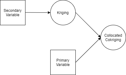
Although in mining and petroleum engineering some variables are collected exhaustively (like seismic data which is measured at the entirety of the subsurface), this method could also be applied by using estimations of the secondary variable at the subsurface as input into Collocated Cokriging. This is the approach that is taken in this project, where Kriging is first implemented on the four variables and then Collocated Cokriging is implemented on the primary variable using the Kriged estimations of the three other variables, which by the nature of Kriging are available at the entirety of the subsurface (figure 03).
Figure 03 - A diagram explaining the conceptual framework of Collocated Cokriging. Estimations of the secondary variable are generated using Kriging and are used as input in the Collocated Cokriging of the primary variable.
Objectives
As stated above, there is a constant effort to improve the quality of spatial estimation methods so that they would yield more reliable results. However, the decision to use which estimation method is often complex, multi-faceted, and most importantly case-specific. One estimation method might perform exceptionally well in one case, whereas the same method might produce erroneous models in another case. As a result, before the actual estimation of the subsurface could be implemented, a comprehensive study must take place to decide which estimation method generates more accurate results in the specific case at hand. Collocated Cokriging, specifically, is a novel method and its effect on different geological settings has not been fully explored. Because of that, it is important to test its capacities for a petroleum data set.
This project is focused on Kriging and Collocated Cokriging and their performance in the project's data set. Four spatial variables are considered: effective porosity (Phie), saturation of oil (SO), effective water saturation (SWE), and bulk mass fraction of oil (BMFO). The primary variable of interest is effective porosity, which represents the capacity of a rock or sediment to contribute to liquid flow. In simpler words, a highly porous rock acts like a sponge and absorbs liquid, which in this setting is oil. This leads to a significant correlation between effective porosity, oil saturation, and bulk mass fraction of oil, which are two variables that directly point to the presence of oil. Effective water saturation is defined as the non-oil liquid saturation, which is almost always water, and has an almost -1.0 correlation coefficient with saturation of oil. The reason that effective porosity is chosen as the target variable in this project is because it gives critical information about flow capacity of rocks and sediments and acts as a basis for designing oil wells. This information is more important than oil saturation or bulk mass fraction of oil in a domain where the presence of oil is already proved.
The three secondary variables have high correlations with the primary variable of interest, effective porosity. This makes them suitable candidates for Collocated Cokriging with effective porosity. Besides, these four variables are some of the most commonly sampled variables at a petroleum project. This enables an extension of the results of this project to similar petroleum cases that also have samples of these variables.
The objective is to estimate effective porosity at the entire domain and to find the more appropriate and effective estimation method. In the first stage, effective porosity is estimated using Kriging. Subsequently, using Kriged values of the other three variables, Collocated Cokriging is performed with each of the other three variables. The results will be compared and analyzed to test which of the two estimation methods is generating more accurate and useful results. The results are also compared between the three secondary variables to see which of them generate better results.
The main criterion parameter is "estimation variance" which quantifies the uncertainty of estimation at each location. As a matter of fact, Kriging results at each point is not a single scalar value, but a full statistical distribution with a mean and variance. The mean of that distribution is reported as the Kriged estimate at that location and estimation variance shows the dispersion of that distribution around the mean. If many samples are used to estimate at a location, then the estimation variance tends to be low, but having very few far-apart samples to inform estimation at a point increases estimation variance. Thus, estimation variance tends to be lower in highly sampled areas and very high in sparsely sampled sections of the domain. But if two different methods generate different estimation variances at the same points, this is indicating that one of them is generating more reliable and less uncertain results.
Expected Results
Collocated Cokriging of a variable utilizes not only samples of that variable at the subsurface, but also uses as input estimations of a secondary variable which is correlated to the primary variable. According to the theory of linear regression, adding additional terms in the estimation equations results in reducing the error, or the estimation variance in case of Kriging. Since an additional term is added in Collocated Cokriging (expression 5), it is expected that Collocated Cokriging generate lower estimation variances. In that case, the main question would be in which areas this reduction of estimation variance is higher. Also based on the theory of linear regression, the stronger the correlation between the response and predictor variables, the lower the error associated with the estimation of the response variable. This implies that secondary variables with higher correlation to the primary variable should generate lower estimation variances in the results.